Variable Sized MoEs

Acknowledgements

Thanks to:

• Sam Lehman for the conversations that got this project off the ground as well as reading drafts and feedback
• Craig Robinson for feedback on drafts
• Andrej Karpathy for NanoGPT, which this project is based on
• Trevor Gale, Deepak Narayanan, Cliff Young, and Matei Zaharia for MegaBlocks, the other foundation for this project

Extending Megablocks with Variable Sized MoEs

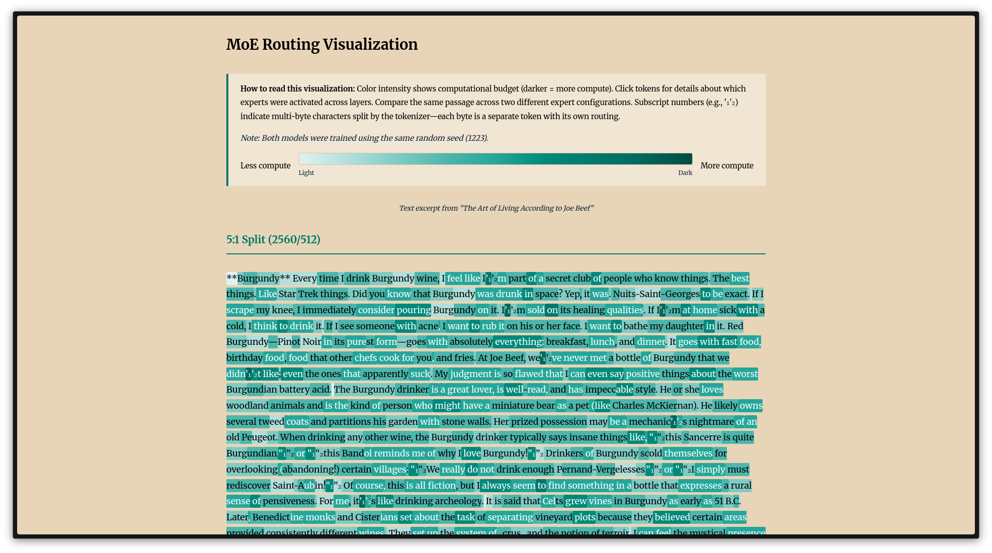
I implemented variable sized experts using Andrej Karpathy’s nanoGPT, which allows us to set the sizes of experts in a mixture of experts (MoE) model. I trained a bunch of variable sized expert MoEs averaging around 125 million active parameters on a chinchilla-optimal ~2.5B tokens. I expected tokens to route based on computational difficulty (something like difficult reasoning to large experts, simple concepts to small ones). It turns out that tokens in constrained contexts like code or recipes route to small experts, and more ambiguous function words like ‘ with’ and ‘ to’ route to larger ones. My interpretation is that large experts handle tokens that need more context to interpret, while small experts handle words with specific meanings. Check out the visualization of where different tokens go here, and code here!

Stage 0: MoE Background

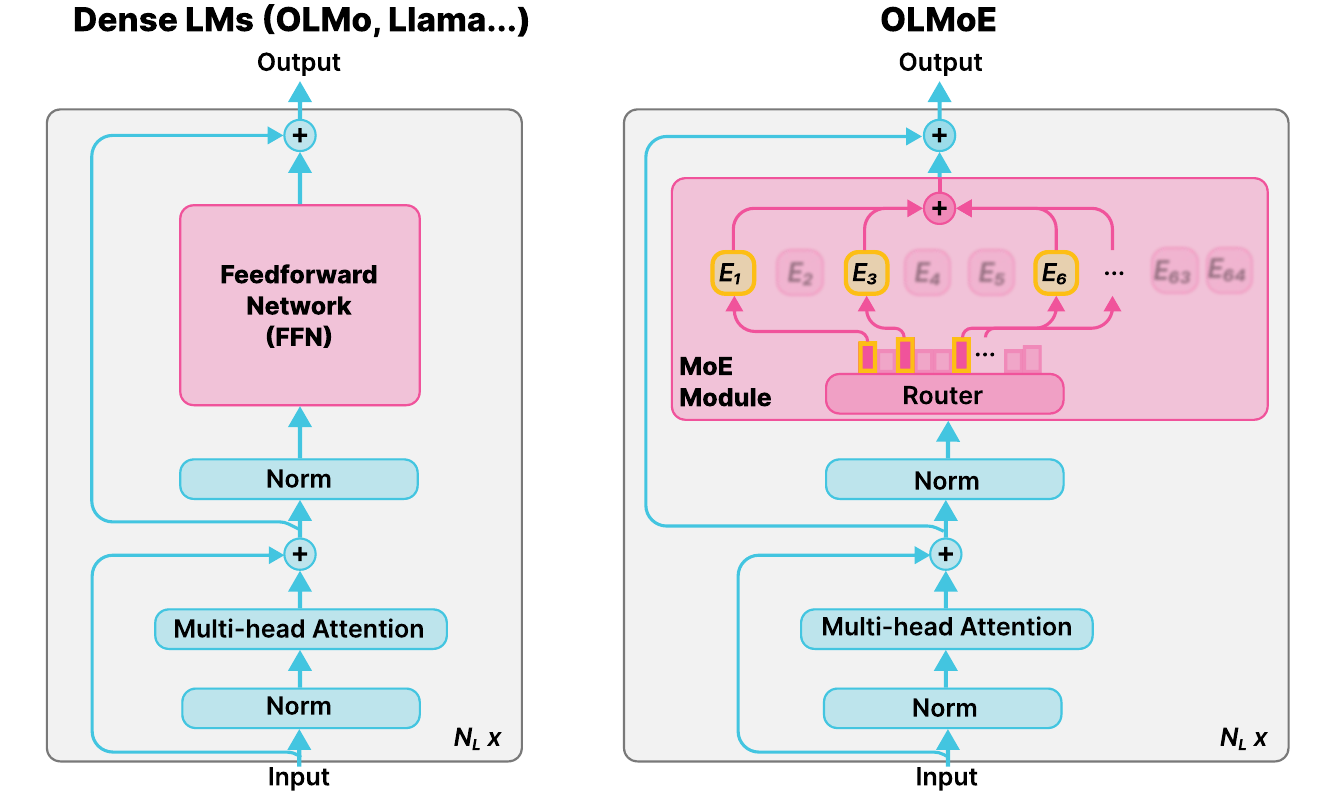
Dense LLMs have a feedforward network (FFN)¹ that every token passes through entirely. MoEs replace this with a much larger layer broken into pieces called “experts”. In an MoE, each token only activates a few experts. This way, MoEs can be more capable, while processing at the same speed.

Historically, MoEs have only been made up of uniform experts of equal size. Here, I explore what happens when we vary the size of the experts. For this project, the ratio (5:1, 23:1) is the size difference between large and small experts. A 23:1 model’s large experts are 23 times the size of its small experts. The two models I trained have the following attributes:

5:1 configuration: Four experts at 2560 hidden dim, four at 512. 2 experts are active². Empirically, active parameters range from 95.7M to 138.7M and we average 114.7M.

23:1 configuration: Four experts at 2944 hidden dim, four at 128 from 91.5M to 114.5M, 101.9M on average.

Record scratch

But first let’s talk about how I got myself into this situation.

Stage 1: Vanilla MoEs

I started this escapade with a simple goal: add efficient³ MoE support to Karpathy’s nanoGPT. I found all the regular things that we’d expect to find with MoEs: they perform better, and for the most part, the sparser, the better. The best performing regular MoE was 64 total, with 8 active (gpt2 wandb, wikitext wandb). It reached a final loss of 3.127 on Openwebtext on a little over chinchilla-optimal 3 billion tokens, compared to 3.285 for the dense model. The 64 total, 8 active model beat the dense model’s loss in 70% of the steps. However, due to (I think) memory overhead, the training run took twice as long (20m for dense vs 40m for the 64x8 MoE). 70% of 40 minutes is 28 minutes, so even if we adjust for hitting the same loss, the MoE doesn’t train as fast at this small scale⁴. In the OLMoE paper, the AI2 team got to the same loss 2x faster compared to the dense model they trained.

This MoE mission opened up a whole, unexpected, gigantic can of worms.

Stage 2: Variable sized experts

Part of the quest of not using for loops led me to MegaBlocks (github and paper). The main MegaBlocks innovation is that we can break matrix multiplications up into blocks of 128, allowing us to avoid dropping tokens when experts get too many, and use less padding when experts get too few. They find that dropping tokens leads to substantially worse performance. The paper goes on to say that “we could also relax the constraint on the number of columns in each block to build MoE layers with variable sized experts”. This, along with conversations with my friend Sam, and two Dwarkesh Patel interviews (Jeff Dean and Noam Shazeer, Sholto Douglas and Trenton Bricken) led me down this rabbit hole of variable sized experts (By no means am I saying that this is exactly what Jeff or Sholto had in mind). Notably, Meituan’s LongCat explores this by using identity experts that route some tokens through zero computation experts. Here, I look at the continuous case: experts of different sizes rather than on/off.
It’s clear that not all tokens are equally hard to predict. So then, why do MoEs have uniformly sized experts? If we can allocate more FLOPs to the harder tokens (whatever that ends up meaning), then maybe we can get a more efficient model⁵. Or maybe we can learn something about what “harder” even means to a model.

So, I started working on this concept, only tweaking MegaBlocks slightly. The fork of MegaBlocks is on my GitHub. I started training some models with variable expert sizes, at first only using a traditional load balancing loss and a router z loss. With a load balancing loss as low as we used for the vanilla MoEs, tokens routed to large experts disproportionately, just as you might think. So, I tried turning up the load balancing loss to get better balance. The best performing vanilla load balancing loss was with an lbl weight of 0.1, a factor of 10 higher than I found was optimal for the vanilla MoEs (wandb). Some great learnings came from that, but these models were well balanced between all the experts, meaning that they routed 50% of tokens to the large experts, and 50% to small. Since I was having the large and the small experts add up to the same intermediate size as the vanilla MoEs, this just averaged the same size of experts as the vanilla MoEs. It performed ever so slightly worse, training in about the same amount of time: not so exciting. We’d need a loss term that lets the model be more free to choose whichever experts it wants.

Stage 3a: Compute balancing loss

This is very similar to our normal load balancing loss. For this, we:

1. Normalize the expert sizes by dividing the expert sizes by the average size of the experts
2. Compute the weighted sum of the router probabilities and the normalized expert sizes (this is a dot product between the router probs and the normalized expert sizes)
3. Take the average of that!

This setup did allow the model to learn to allocate different size experts to different tokens. Both the 5:1 and 23:1 models ended up at around 70% small and 30% large experts. After training, there were still load imbalances within groups of experts, so we needed to add slightly modified load balancing loss back in.

Stage 3b: Group load balancing loss

This is pretty simple: we just divide up the expert groups, and use the same load balancing loss that we used above and got from OLMoE. This new scheme balanced well at weight 0.01.

So now, I’d done it! We have variable sized MoEs and can train a bunch of size ratios.

Stage 4: Training a bunch of these models

I started on a smaller model size to sweep over the size ratios, training roughly 50M active models on Wikitext. The most promising runs were at 4:1, 6:1, and 19:1 (large:small). The 19:1 used the smallest experts MegaBlocks allows: 128 hidden dim. The 19:1 model finished training in 84% of the time with only 3.2% higher loss. The 4:1 finished in 91% of the time with 0.96% higher loss; the 6:1 in 89% with 1.4% higher.

So, with the hypothesis that something around 4:1 or 6:1 would be the optimal “larger” ratio and the extreme “smaller” ~19:1 ratio in mind, I went up to GPT-2’s size of about 125 million active parameters. I stuck with openwebtext as a fair comparison to the original models I trained. I trained the final models with a load balancing loss weight of 0.08, and a compute loss weight of 0.004⁶. I found very similar results across the board: the extreme ratio (this time 23:1, again with small experts of size 128) was much faster to train, this time with a 20% speedup and a 2.5% loss degradation. The average size of experts in evaluation was 861. The more moderate 5:1 ratio was 10% faster, with 0.5% loss degradation, with an average size of 1077.

One ablation I ran was with consistently sized experts, but much smaller than 1536. I chose 896 because it was the closest multiple of 128 to our 861 average size. Bluntly, this run was disappointing to me: it beat all but the 5:1 ratio on loss, and finished training faster than the 23:1 ratio runs, though they were within spitting distance of each other (Update: a couple weeks later after going over my routing layer by layer, I noticed that the first layer was extremely imbalanced within size groups. Fixing this for 23:1 runs actually ended up matching the loss and speed. I think the takeaway is still the same though). This shows us that the active MLP width need not be 4*hidden size. We already see this in most of the best-performing open source MoE models: Deepseek V3 and Kimi K2 (which both use Deepseek’s basic architecture) use experts that add up to an expansion factor of ~2.57, and GLM-4.6 uses 2.7. (Minimax M2, gpt-oss and OLMoE all use 4x).

Efficiency aside, this was the real question I wanted to answer: do the models learn meaningful routing patterns?

Stage 5: contextual ambiguity, routing analysis, domain specialization, and syntactic specialization

This was what I was most excited about: do experts actually specialize? There have been conflicting reports. The original MoE paper uses LSTMs and tons and tons of experts (up to 131,072!), and shows clear specialization. Then, the ST-MoE paper shows that the encoder specializes, but “expert specialization is far less noticeable in the decoder” (recall that most of the generative models that we think of are decoder only). The Mixtral paper shows no domain specialization at all, but does find syntactic specialization⁷. OLMoE shows that certain tokens, like those from arxiv, consistently route to certain experts. Finally, Deepseek MoE) makes the claim that their MoE performs better than GShard due to more expert specialization. Their focus is mostly on redundancy across experts, not individual token routing analysis or domain specialization. All of this is ok evidence that there probably is some kind of specialization going on with MoEs, but not conclusive at all. My holy grail would be to one day figure out that specialization and show that if we turn off certain expert combinations across layers (say, if there are experts that get lots of code tokens), performance tanks. Additionally, if we isolated those experts into a dense model, would we be able to keep the performance in that area? To me, this would be the clearest evidence that the experts do specialize. I don’t achieve this here.

The 23:1 and 5:1 models learn pretty different routing schemes. For starters, the 5:1 ratio has a 0.295 spearman correlation⁸ between the token count in the dataset and the average size of the expert. On the other hand, for the 23:1 ratio, we see a negative correlation: -0.222. So, I’ll break them into two sections. I expected that because of the extreme difference in experts, we’d see a clearer pattern. That doesn’t seem to be true. The 5:1 model’s highest vs lowest expert sizes is actually larger than the 23:1 model’s (the delta is 2332 for 5:1 and 1252 for 23:1). The average size of the experts and entropy for the 5:1 ratio are not at all spearman correlated (literally 0.00), and the 23:1 is weakly negatively correlated (-0.150). So what are they even learning?

I think the models I’ve trained here learn the contexts that they are in: when they are in a constrained context like programming, a recipe, or finishing a common word, they tend to use smaller experts. When the context is more ambiguous, they use larger experts.

If we look at different counts of tokens, we see that the two ratios learn different patterns by frequencies. When we get to more frequently occurring tokens, there is higher correlation between the two mean sizes, meaning that there is some (small) relationship between the sizes that the two learn (see the table below). So they don’t learn totally orthogonal patterns, but they definitely learn different ones. For example, “ing” words go to large experts for 5:1 and small for 23:1. Let’s take a closer look at the patterns.

Token Frequency Range	Number of Samples (n)	Spearman Correlation
(0, 10]	20,975	-0.0740
(10, 50]	18,218	-0.0840
(50, 100]	3,825	-0.0209
(100, 500]	3,657	0.0853
(500, 1000]	514	0.1132
(1000, 5000]	318	0.2874
5000+	77	0.1257

5:1

We see a pretty clear pattern with the 5:1 model, especially on the low average expert size end.
Technical tokens like “ goto”, “ perl”, and “ println” are all at the low end of the compute spectrum. There are the second halves of somewhat unique words like “oenix”, “ibrary”, and ”chnology”. We also see “ tbsp”, “ teaspoons”, and “ tablespoons”, as well as “ lol” and “ haha”. Additionally, we see discourse markers like “Furthermore”, “Moreover”, and “Similarly”. These are all capitalized! When we look at the lowercase versions of these tokens, we see that they actually use larger experts. Most extremely, “ similarly” is actually in the top 2400 out of around 50 thousand. It’s particularly syntactically ambiguous: there are a bunch of different ways to use the word. When it’s at the start of the sentence, chances are very good that it’ll be referring to the previous sentence.

On the other end of the scale, the tokens that use the largest experts are the token ids <564> and <447>. These are the only tokens that use larger experts on average than our baseline⁹.

Now, if we try to decode these tokens just in the python interpreter, they don’t print correctly. That’s because they are both incomplete byte strings– some token comes after them. So, decoding them as bytes, we see that 447 is ‘e280’, and 564 is ‘20e280’. It turns out that ‘20’ is just a space, so 564 is basically ‘ e280’. If we dig deeper, we see that e2 80 is the beginning of 64 different types of punctuation including “—” (em dash), “‡” (double dagger), and my favorite, “‽” (interrobang) (see full list here), along with a bunch of different spaces. Another fascinating thing about these tokens is that they get down to a very low entropy. Since there are only 64 options that can follow the ‘e280’ bytes or else there will be a catastrophic failure, the model seems to learn that it only really has 64 options, leading to the low entropy. Then, it needs big experts to decide which of the 64 possible tokens come next, since there’s a lot of ambiguity for which symbol should come next. Also appearing on the high side: function words like “ with”, “ to”, and “ in”.

What I think is going on: these models are routing tokens based on contextual constraint—when what comes next is predictable, they use less compute. Within the low compute regimes, the context is very constrained. For example, with the technical words, there are only so many things that can come after “ println”, or with “ tbsp”, we’re almost certainly in a recipe setting. Lastly, with the discourse markers, I think they kind of ‘tell you what’s coming’: another, similar point.

23:1

As I said above, this model’s routing patterns are pretty different. It’s slightly negatively correlated with token occurrences in the dataset, and again very slightly negatively correlated with the output entropies (-0.15). The two aren’t correlated with each other. There are patterns at the low end: we see lots of names and other proper nouns “ Abraham”, “Stephen”, “ Jon”/“John”, “ Obama”. There are some code-related tokens as well like “ !=”, “ ();”, and “ ()”, and a lot of numbers. At the high end, it’s a lot more of a grab bag, but we do see some similar word endings and whole words (though I feel like I’m trying to cram my previous observations onto this). We do see token 564 show up again, and 447 is in the upper quartile.

Domain Specialization

Joining the two ratios back together, I tested domain specialization by running both models on different domains from the Dolma 3 pool. The only meaningful domain effect for this setup is code.

For the 5:1 model, code’s weighted average expert size is 2244, which is 210 smaller than the 2454 size observed across all other domains. The 23:1 model is even more extreme: code drops to 1499 vs 2131 for other domains, a gap of 632. This is 14.3 standard deviations below the cross-domain mean! When given more dynamic range, the model leans harder into treating code as low-compute. Code’s maximum expert size is 2958 (5:1) and 2916 (23:1), while natural language domains reach 3697-3755. Of 690 tokens appearing across all domains with count >100, 518 route lower in code and only 165 route higher (the remaining 7 were the same). Tokens like “ is”, “ in”, and “ return” (all programming keywords) drop 250-450 in code. But the pattern flips for subword fragments: short tokens like ‘ker’, ‘ame’, and single characters route higher in code, since they could be part of any identifier.

The other domains cluster together. Politics and crime & law route slightly higher (+30 and +26 vs the cross-domain mean), sci_math_tech slightly lower (-31), but this ~60 point spread is noise compared to code’s ~600 point gap in the 23:1 model.

Wrapping up, Open Questions

At this scale, we don’t see any efficiency gains other than what you’d get from only using smaller experts. Routing is consistent across seeds: function words go to big experts, and code goes to smaller ones. I expected “difficult” tokens (code, math, technical terms) to get more compute; that’s not what happens in my experiments.

Open questions and things I want to try next:

1) I haven’t yet trained many models with better-performing expert setups than 8x2 (eg 64x8). The size differences with more experts were less extreme, so I thought 8x2 would be more revealing to study.
2) Imbalanced expert counts, shared experts. Deepseek V3 and other models based on its architecture, like Kimi K2, use a shared expert, one expert that’s always active. Could we use one large expert as the shared expert, and the rest small experts, or something like this idea? Is there an optimal number of experts of each size (something like, without loss of generality, 2 large, 6 small)? Could we do small, medium, and large?
3) FlexOlmo worked on the concept of training dense models separately and then stitching them together – could we use these variable sized experts to have smaller specialized experts with a larger, more general model as the backbone?
4) Beat the baseline by tuning the compute balancing loss coefficient
5) How’s this stuff interact with attention scores? Especially with the discourse markers thing. Perhaps a “Moreover” token is attending to the last sentence quite a lot and this lines up with the lack of compute?
6) Intermediate ratio analysis– is there a crossover point somewhere between the 5:1 and 23:1 where we see the correlations flip?
7) This last weekend (Dec 13/14 2025) I tried subbing in a sigmoid instead of softmax for routing, like they do in DeepSeek-V3. It learned more like an 80:20 small:large ratio. I haven’t had a chance to look at the routing. Will everything we saw above hold?
8) RL’s been used for gating– obviously that hasn’t stuck around. Would it help us allocate our compute better in some way?